How-To
How to Optimize Treatment Timing
Most infrastructure assets deteriorate over time, either through use or weathering, passing through different stages of condition as they age. Assets in more advanced stages of deterioration generally require more extensive and expensive treatments. The period during which a treatment is recommended to address deterioration is referred to as the treatment’s “window of opportunity.” The following figure, from the 2023 New York State Department of Transportation (NYSDOT) TAMP illustrates windows of opportunity for pavement assets.
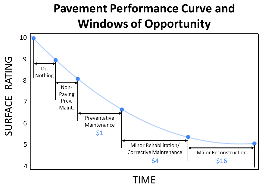
Source: 2023 New York State Department of Transportation TAMP.
Windows of opportunity are treatment-specific. As demonstrated in the figure, the window of opportunity for a preventive maintenance overlay is approximately one third the length of a mill and inlay’s window. As explained in NYSDOT’s TAMP, “The dollar amounts shown in [the figure] represent the ratio of typical costs between treatments that are appropriate in each window of opportunity.”
If a treatment is delivered too late, its service life may be significantly shortened. If a treatment is delivered too early, then benefits from prior treatments may be lost. In most cases, delivering a treatment in the beginning of its appropriate window is more efficient than deferring it to the end. Slow delivery may reduce service life while increasing the risk of missing the window entirely. To improve timing, it is necessary to consider the expected duration of treatment development and delivery phases. While some treatments may be delivered within weeks, others may take years of planning, design, and procurement.
Beyond delivering a treatment within the proper window of opportunity, the optimal timing of a treatment can be evaluated through analysis of benefit and cost. There are many different approaches to this benefit-cost (b/c) analysis. Below are two examples of varying complexity.
Remaining Service Life (RSL) Evaluation
Agencies with an understanding of the service lives for its treatments can use the concept of remaining service life to understand the best mix of treatments either at the present time or over the course of a given planning horizon. The approach is based on the premise that each asset loses one year of service life for each year in service. With some basic information, an agency can determine the best balance of investments across treatment types to minimize future costs. This information typically includes:
- The appropriate treatment for an asset, given its age or condition.
- The remaining years in its current window of opportunity.
- The cost of each treatment.
This approach will often lead to maximizing the application of lighter treatments to avoid the need for more extensive and expensive treatments. The National Center for Pavement Preservation (NCPP) has developed an approach to RSL evaluation for pavements. Additional information, and a free analysis tool can be found on the NCPP website.
Maximizing Benefit Over Time
NCHRP Report 523 provides a process for optimizing the timing of pavement preservation using benefit cost analysis. Most commercial asset management systems use some variation of this modeling approach. Although the original research, and the examples below, are based on pavements, it can be applied to other assets. By iteratively performing the following steps at different points in time, an optimal treatment timing can be determined through the model (NCHRP 2004).
Analysis Setup
Develop a catalog of relevant treatments, windows of opportunity, and measures of benefit.
Selection of Benefit Cutoff Values
Determine thresholds for benefit measures where the agency will see diminishing returns. For example, if the agency determines that an International Roughness Index (IRI) value of 60 inches per mile is excellent, and a given treatment is determined to decrease IRI to 50 inches per mile, there will be no additional benefit modeled for a treatment that improves ride from 60 to 50 inches per mile.
Computation of Area Associated with the Do-Nothing Case
Calculate the area bounded by the upper cutoff, lower cutoff, and the expected performance curve. The following figure provides an example of calculating the benefit of a do-nothing treatment for a performance measure that increases with age, e.g., IRI.
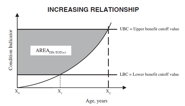
Source: NCHRP 2004
Computation of the Overall Expected Service Life of the Do-Nothing Case
Estimate the number of years before the asset reaches a failed condition state without treatment.
Computation of Expected Service Life of the Post-Treatment Case
Estimate the number of years before the asset reaches a failed condition state after the treatment. This is illustrated for IRI in the following figure.
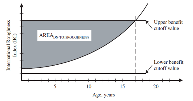
Source: NCHRP 2004
Computation of Areas Associated with the Post-Treatment Case
Calculate and compare the post treatment area with the do-noting area to determine the net increase in benefit. A graphical example of this net benefit area is shown in the figure below.
